It has been discussed that many types of unstable modes appear in equatorial regions of atmosphere and ocean. Dunkerton (1981) and Stevens (1983) showed that, with shallow water models on an equatorial β-plane, zonally symmetric inertially unstable modes appear if there exists the inertially unstable region defined as a region where the product of the Coriolis parameter and potential vorticity is negative. Dunkerton (1983) showed the existence of zonally nonsymmetric modes with large amplitudes in inertially unstable regions. Natarov and Boyd (2001) discussed that equatorial Kelvin wave (Matsuno, 1966) is destabilized in equatorial shear flow.
Taniguchi and Ishiwatari (2006, hereafter TI2006)
reconsidered the above mentioned unstable modes
from the viewpoint of the concept of
resonance between neutral waves
(Hayashi and Young, 1987;
Iga, 1999c).
TI2006
obtained unstable modes of a linear shear flow in a shallow water
on an equatorial β-plane over a wide
range of nondimensional parameter
 ,
where
,
where
 ,
,
 ,
,
 ,
and
,
and  are the meridional shear of basic zonal flow,
gravitational constant,
equivalent depth,
and the north-south gradient of the Coriolis parameter, respectively.
are the meridional shear of basic zonal flow,
gravitational constant,
equivalent depth,
and the north-south gradient of the Coriolis parameter, respectively.
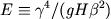
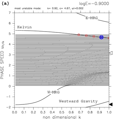
TI2006 classified the resonance types of the most unstable modes according to the value of E as summarized in table 1 (see animation figure for the cases not shown in table 1). They showed that the nonsymmetric unstable modes of Dunkerton (1983) and symmetric inertially unstable modes (Dunkerton, 1981; Stevens, 1983) are the same kind of instability caused by the resonance between equatorial Kelvin modes and westward mixed Rossby-gravity modes (Matsuno, 1966). It was also shown that the destabilized equatorial Kelvin wave obtained by Natarov and Boyd, 2001 corresponds to unstable modes caused by resonance between equatorial Kelvin modes and continuous modes (Case, 1960).
| range of E | log E < 1.00 | 1.00 < log E < 2.00 | log E > 2.00 |
| dispersion curves |
|
|
 |
| most unstable mode structure | nonsymmetric structures | nonsymmetric structures | symmetric structures |
|
resonance type of most unstable modes |
equatorial Kelvin modes and continuous modes |
equatorial Kelvin modes and west- ward mixed Rossby-gravity modes |
equatorial Kelvin modes and west- ward mixed Rossby-gravity modes |
|
corresponding previous studies |
destabilized equatorial Kelvin wave (Natarov and Boyd, 2001) |
zonally nonsymmetric unstable modes of Dunkerton (1983) |
inertially unstable modes (Dunkerton, 1981; Stevens, 1983) |
Table 1: A summary of interpretation of most unstable modes obtained by TI2006. Values of log E are (a) -0.90, (b) +1.30, (c) +2.50. Upper figure shows dispersion curves for each value of E. Click figures of dispersion curves to show larger figures. Horizontal and vertical axes are non-dimensional zonal wavenumber and phase speed (c), respectively. The labels 'Kelvin', 'E-MRG', 'W-MRG', 'Eastward Gravity', and 'Westward Gravity' indicate equatorial Kelvin modes, eastward mixed Rossby-gravity modes, westward mixed Rossby-gravity modes, eastward inertial gravity modes, and westward inertial gravity modes, respectively (refer to Matsuno (1966) for each mode). The label 'Kelvin + W-MRG' indicates unstable modes caused by resonance between equatorial Kelvin modes and westward mixed Rossby-gravity modes. Horizontal lines in the range of 0.00 < c < 5.00 are dispersion curves of continuous modes. Open red circles and double blue circles indicate unstable modes and the most unstable modes, respectively. Open and filled triangles indicate the position of dispersion curves of north and south boundary Kelvin modes, respectively. The third and the fourth rows show horizontal structure of most unstable modes and resonance types, respectively. The bottom row shows the corresponding previous study for each most unstable mode.