Introduction

Open-ocean deep convection is a phenomenon in which vertical water movements penetrates well below the surface mixed layer caused by surface buoyancy loss in open ocean. The "open-ocean" means that the convective phenomena are not significantly influenced by lateral boundaries. Open-ocean deep convection supplies dense waters, which play a significant role in the earth's heat transport and hence heat balance.

Numerical simulation of open-ocean deep convection has been studied by a number of papers (see Marshall and Schott (1999) for a review) after the pioneering work by Johns and Marshall (1993). The oceanographic deep convection have different physical parameter ranges from those in the atmospheric convection as noted by Klinger and Marshall (1995) (hereafter KM); the atmospheric convection hits the ceiling (tropopause) before it feels the effect of rotation, but the open-ocean deep convection feels the earth's rotation before convective elements reach the ocean bottom. Therefore, the oceanic deep convection forms a relatively new class of convective problems in geophysical fluid dynamics.

A convection phenomenon usually occurs in a wider area than the ocean depth, and the spatial domain where convection occurs is called convection patch whose diameter is a few tens of kilometers. The water movements in a convection patch is characterized by a number of plumes, whose diameter is typically several hundreds meters. The plumes are convective elements that moves vertically, and play substantial roles in vertical water mixing in the convection patch.

Previous numerical and laboratory studies have shown that plumes exhibit qualitatively different two regimes, which are referred to as a two dimensional (2-D) and three dimensional (3-D) regimes. In a 2-D regime, velocity fields are dominated by the first vertical mode. Thus, the terminology, 2-D regime, comes from the fact that one can approximately know a whole (three dimensional) flow field by obtaining one horizontal cross section (one 2-D plane, i.e., at a quarter depth) and the fixed vertical structure. On the other hand, in a 3-D regime, the vertical structures of the current fields vary spatially and temporally, and hence one cannot extract a dominant single vertical structure. KM proposed that the 2-D and 3-D regimes can be uniquely separated by a line in a two dimensional logarithmic parameter space of flux Rayleigh number and natural Rossby number. However, because the number of the KM's experiments (19) is not enough to determine whether or not the separation line is a part of a more complex curve. In order to address this question, we have conducted a larger number of numerical experiments (157).

The mechanism separating the 2-D and 3-D regimes is not clear. We examine this problem from a point of view of the entropy increase rate of the system. It is known that behaviors of some complex systems are explained by the maximization hypothesis of entropy increase rate. The hypothesis states that the behavior of the system is adjusted so as to maximize the entropy increase rate. The hypothesis has been successfully applied to a number of phenomena, which have various time and spatial scales, i.e., the earth's climate (e.g., Paltridge 1975, Ozawa and Ohmura 1997) and frost heaving (Ozawa 1997). In particular, for a system that has possible different regimes corresponding different entropy increase rates, a regime which has a larger entropy increase rate than others should be selected in reality, as far as the maximization of the entropy increase rate is applicable (Sawada 1981). A conceptual example of the hypothesis for multiple regimes is illustrated in Fig. 1. Thus, if the 2-D and 3-D separation is consistent with the hypothesis, the entropy increase rate should exhibit gradients shown in either left or right panel in Fig. 1. We will examine whether this is the case or not. Such approach examining the entropy is a macroscopic approach, which would play a complementary role to microscopic approaches in understanding the regime transition. An example of the microscopic approach is employed by KM, who suggested that the instability of the first vertical mode in the 2-D regime causes the transition from the 2-D regime into the 3-D regime.

In addition to the problems associated with the 2-D and 3-D regime transition, we will examine the structures of the plumes in the 2-D regime. Sometimes, the 2-D regime is assumed to be characterized by quasi-stable vortex pairs rotating different directions in the top and bottom of the fluid. Such a stable vortex pair is called as a heton. For example, KM called the 2-D regime the heton regime. However, it is not still clear whether or not the major structures of all 2-D regimes are hetons. In the present paper, therefore, we investigate the flow structures in the 2-D regime in more detail than in the previous studies by employing visual inspections of vorticity and velocity structures including animations. Apparently, the present journal, Nagare Multimedia, has great advantages for the visual inspection of time varying complex structures over conventional paper journals.

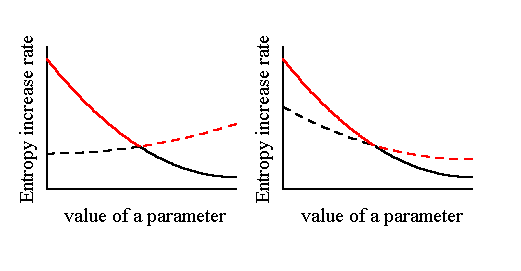
Figure 1. Schematic explains how a regime, which has a larger entropy increase rate than the other potentially possible regime, is selected. The solid and dashed curve indicates the entropy increase rate in a two potentially possible regimes as a function of a parameter value. A regime having a larger entropy increase rate (red solid or red dashed curves) should be selected to occur in reality, as far as the maximization hypothesis of entropy increase rate can be applicable to the system. The left panel is the case where the entropy increase rate has its minimum at the transition point between the two regimes. However, the occurrence of the minimal value is not necessary as illustrated in the right panel, where both the entropy increase rates of the two regimes are given by the decreasing functions of the parameter.