| SPMODEL: A Series of Hierarchical Spectral Models for GFD | << Prev | Index| Next >> |
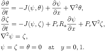
This is a Boussinesq fluid model of thermal convection that occurs in a fluid layer between parallel horizontal planes uniformly heated from below and cooled from above. The governing equations are the vorticity equation and the equation of temperature disturbance in a two-dimensional channel domain of a Boussinesq fluid.

ψ is the stream function, ζ is vorticity, and θ is temperature disturbance from the basic state. The first terms on the right-hand side of the first and the second equations J(ψ,θ), J(ψ,ζ) are the Jacobian; they describe the advection of temperature and vorticity, respectively. The fourth equation is the boundary conditions on the upper and lower horizontal plane; it expresses the free-slip and fixed temperature boundary conditions. The detailed formulation and linear stability analysis of this system are explained in textbooks of fluid mechanics (such as [10]) or [11].
The resulting program source code is given as bsncnv-tt-2.f90. As eigen function series satisfying the boundary conditions, the usual Fourier series in x direction and Fourier sine series in y direction are employed, respectively. The main part of the time integration is as follows:
do it=1,nt
    es_TempA = es_TempB + &
              dt*( -es_Jacobian_es_es(es_PsiB,es_TempB) &
                    + es_Dx_es(es_PsiB) &
                    + es_Lapla_es(es_TempB) )

    es_ZetaA = es_ZetaB + &
              dt*( - es_Jacobian_es_es(es_PsiB,es_ZetaB) &
                    + Pr*Ra*es_Dx_es(es_TempB) + Pr*es_Lapla_es(es_ZetaB)    )

    es_PsiA = es_LaplaInv_es(es_ZetaA)

    es_TempB = es_TempA
    es_PsiB  = es_PsiA
    es_ZetaB = es_ZetaA
    ...
enddo
The prefix "es_" and the suffix "_es" denote the spectral data whose first dimension is the usual Fourier series component and second dimension is the Fourier sine series component. Time integration is performed by the Euler scheme. The last character "B" in the variable names means that the variables are for the present time step (abbreviation of "Before"), and "A" means the variables for the next time step (abbreviation of "After").
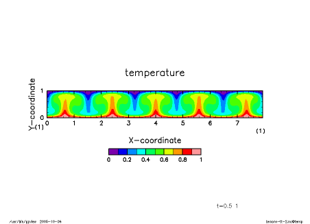
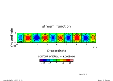
Numerical results starting from a pointwise temperature disturbance placed initially near the center of the domain are shown below. The Rayleigh number Ra, and the Prandtl number Pr are 10000 and 1, respectively. Development of convection cells with aspect ratio nearly equal to unity can be observed.
|
| [animation] | [animation] |
It is known that the thermal condition at the boundaries affects the structure of convection ([11]). When the fixed heat flux condition is adopted instead of the fixed temperature condition used above, we obtain the following equation as the boundary conditions:

The whole program source code is given as bsncnv-ff-1.f90. In order to satisfy the thermal condition, the temperature disturbance field is now expanded by the Fourier cosine series in the y direction. The stream function and vorticity fields are expanded by the Fourier sine series, as in the previous example. The main part of the time integration is as follows:
do it=1,nt
    ec_TempA = ec_TempB + &
            dt*( - ec_Jacobian_es_ec(es_PsiB,ec_TempB) &
                 + ec_yx(yx_es(es_dx_es(es_PsiB)))  &
                 + ec_Lapla_ec(ec_TempB) )

    es_ZetaA = es_ZetaB + &
            dt*( - es_Jacobian_es_es(es_PsiB,es_ZetaB) &
                 + Pr * Ra * es_yx(yx_ec(ec_Dx_ec(ec_TempB))) &
                 + Pr * es_Lapla_es(es_ZetaB)    )

    es_PsiA = es_LaplaInv_es(es_ZetaA)

    ec_TempB = ec_TempA
    es_PsiB  = es_PsiA
    es_ZetaB = es_ZetaA
    ...
enddo
The prefix "ec_" and the suffix "_ec" denote the spectral data whose second dimension is the Fourier cosine series component. The prefix "yx_" and the suffix "_yx" represent two-dimensional grid data whose first and second dimensions are components of y and x coordinates, respectively. Since the spectral basis functions of temperature and flow fields are different, conversion of the spectral basis functions is performed by transforming back to the grid data of the real space once.
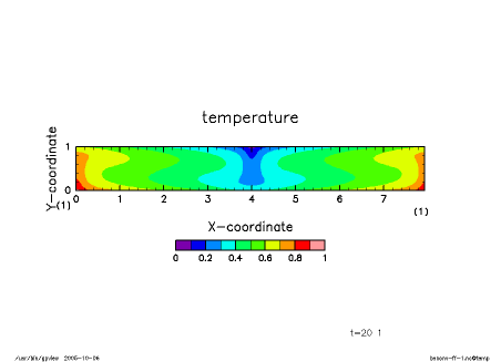
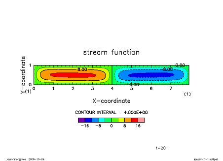
Numerical results starting from the same initial condition as that of the fixed-temperature case are shown in the figures below. As described in [11], convection cells with aspect ratio of about unity become unstable and develop in the early stage of integration, while horizontally elongated convection cells emerge and eventually become dominant.
|
|
| [animation] | [animation] |
| SPMODEL: A Series of Hierarchical Spectral Models for GFD | << Prev | Index| Next >> |