5.4. A shallow water model on a two-dimensional rotating sphere

SPMODEL: A Series of Hierarchical Spectral Models for GFD << Prev | Index| Next >>

5.4. A shallow water model on a two-dimensional rotating sphere

This is a replication of the numerical calculation by [12] where the orographic responses of the atmosphere are considered by the use of a shallow water model on a rotating sphere. What follows is a case presented as an ideal orographic response, where global propagation of waves is caused by an isolated mountain whose radius is 45 degrees located at 30 degree latitude North and 180 degree longitude placed in westerly wind (eastward flow) with rigid rotating distribution.

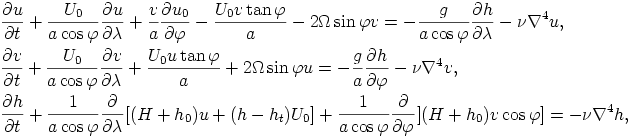
The governing equations are the linearized shallow water model on a rotating sphere:

where U₀ is the given longitudinal velocity of the basic state (rigid rotation), u,v are velocity field disturbances, and H,h and h_t are the averaged fluid depth, surface height, and the bottom topography, respectively. Ω is the rotation rate of the system, ν is the coefficient of the fourth order hyper-viscosity. a is the radius of the sphere, and λ and φ are longitude and latitude, respectively.

The resultant program source code is given as spshallow_topo_linear.f90. Since the computational domain is the whole spherical surface, we use the spherical harmonic series as the basis of spectral expansion. The main part of the program corresponding the governing equations is as follows:

do it=1,nt
    w_U = ( w_U &
        + dt * w_xy( - xy_U0 * xy_GradLon_w(w_U) / R0   &
                     - xy_V  * xy_GradLat_w(w_U0) / R0  &
                     + xy_U0 * xy_V * tan(xy_Lat) / R0  &
                     + 2 * Omega * sin(xy_Lat) * xy_V   &
                     - Grav * xy_GradLon_w(w_H)/ R0   ) &
                     )/(1+Nu*(-rn(:,1)/R0**2)**(ndiff/2)*dt)

    xy_U = xy_w(w_U)

    w_V = ( w_V &
        + dt * w_xy( - xy_U0 * xy_GradLon_w(w_V) / R0   &
                     - xy_U * xy_U0 * tan(xy_Lat) / R0  &
                     - xy_U0 * xy_U * tan(xy_Lat) / R0  &
                     - 2 * Omega * sin(xy_Lat) * xy_U   &
                     - Grav * xy_GradLat_w(w_H) / R0 )  &
                     )/(1+Nu*(-rn(:,1)/r0**2)**(ndiff/2)*dt)

    xy_V = xy_w(w_V)

    w_H = ( w_H &
        + dt * ( - w_Div_xy_xy( xy_U*(H0+xy_H0)+xy_U0*(xy_H-xy_Htopo),   &
                                xy_V*(H0+xy_H0) ) / R0      ) &
                )/(1+Nu*(-rn(:,1)/R0**2)**(ndiff/2)*dt)

    xy_H = xy_w(w_H)
    ...
enddo

The prefix "w_" and the suffix "_w" denote the spectral data expanded by the spherical harmonic series, and the prefix "xy_" and the suffix "_xy" represent the grid data whose first and second dimensions are longitude and latitude, respectively. As for the time integration, the implicit scheme is applied to the viscous terms, while the explicit scheme (the Euler scheme) is applied to the others. -rn(:,1) is the array storing the total wavenumber n(n+1), which is the multiplying factor of the Laplacian operator.

The pictures below show time the development of vorticity field on different map projections. It can be seen that the disturbance is propagating as Rossby waves along the great circle.


[animation]	[animation]