C. Details of the Model

c. Examination on the Vertical Resolution

In this section, we examine the vertical grid resolution that is necessary for radiation calculations. Through comparisons of 1D calculation results obtained from the use of various vertical grid resolutions, the minimum vertical grid resolution required for radiation calculations will be identified.

Positions of the Vertical Layers

Nakajima et al. (1992) conducts calculations using 400 to 700 vertical layers in order to acquire 1D radiative equilibrium solutions. However, it is practically infeasible to conduct 3D time evolutions with that number of vertical grid resolutions. In order to conduct 3D calculations, it is necessary to identify the minimum number of vertical layers that allows radiation calculations with sufficient accuracy. To accomplish this, we will compare calculations from four scenarios: 16, 21, 32, and 1000 vertical layer resolutions. The models based on these four resolutions will be referred to as L16, L21, L32, and L1000, respectively. Table 1 shows the positions of the vertical layers for the case of L32.
In L16, the 15 lowest layers listed in Table 1 are used , and the 16th layer is set to 0. In L21, σ= 10^-1, 10^-2, 10^-3, 10^-4, and 10^-5 are added to the vertical layers of L16. In L1000, the entire atmospheric layer (σ = 1 to 10^-6) is divided into equal intervals of ln p.

Incidentally, the entire atmospheric layer is divided into equal intervals of ln p in Nakajima et al. (1992). In their study, the number of the vertical layers is set to

$\begin{displaymath} NNL = \frac{p_{bottom} - p_{top}}{\ln 10 /100} + 1\end{displaymath}$

The actual numbers of vertical layers are 560 for c_pv = 4R, c_pn = 3.5R, p_n0 = 10⁵ Pa, T_g = 500 K and 702 for c_pv = 4R, c_pn = 4.5R, p_n0 = 10⁸ Pa, T_g = 500 K.

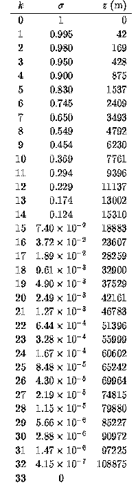
Table 1: Positions of the vertical grids. k: the vertical grid number, numbered in order 0, 1, 2, ... from the surface up. σ :the value of the σ-coordinate. z: the global mean values of the geopotential heights (m) obtained from the case of S = 1380 W/m².

Tg-OLR Relationship

Here, it will be determined if an accurate relationship between T_g and OLR can be obtained with various vertical grid resolutions.

Figure 1 illustrates the relationships between surface temperature and OLR that were acquired for various vertical resolutions for the case of p_n0 = 10⁵ Pa.

The dependency of OLR on Tg in the case of L32 is identical to that in the case of L1000. However, when the resolution is reduced to L21, the T_g-OLR curve becomes undulating. Since this case does not allow an accurate evaluation of the tropopause height, radiative flux cannot be accurately calculated. When the vertical resolution is further reduced to that of L16, no range exists in which the T_g-OLR curve is characterized by a flat line. Such a result is obtained because the top of the troposphere is situated at an altitude higher than the top of the model domain at values of T_g exceeding 350 K. Although the highest layer corresponds to σ= 0.05 in the case of L16, the altitude of the tropopause becomes even higher than this layer when T_g exceeds 350 K.

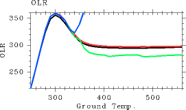
Figure 1: The relationship between surface temperature (K) and OLR (W/m2) for C_{Δ
τ} = 0.1. For the case of p_n0 = 10₅ Pa. Black: the results from L1000. Red: the results from L32. Green: the results from L21. Blue: the results from L16.

For the purpose of comparing these values between the cases of L32 and L1000, Tables 2 and 3 show the values of the OLR from the flat portion and near the peak of the T_g-OLR curve, respectively. The difference in the pairs of values between L32 and L1000 is as large as approximately 5 W/m². Thus, it can be claimed that radiation calculations can be conducted with L32 with an accuracy of approximately 5 W/m².

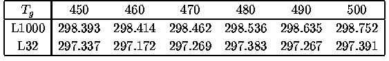
Table 2: The values of OLR from the flat portion of the surface temperature-OLR curve . The values in the rows labeled L1000 and L32 are the values of OLR (W/m²) obtained from setting the number of vertical layers to 1000 and 32, respectively.

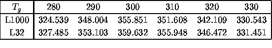
Table 3: The values of OLR from near the peak of the surface temperature-OLR curve. The values in the rows labeled L1000 and L32 are the values of OLR (W/m₂) obtained from setting the number of vertical layers to 1000 and 32, respectively.

The discussions above reveals that L32 allows calculations of OLR with sufficient accuracy for the case of p_n0 = 10⁵ Pa. The subsequent examination addresses whether 1D equilibrium solutions can be accurately obtained when partial pressure of the non-condensable constituents at the surface is varied. Figure 2 shows the T_g-OLR relationship evaluated with L32 for various partial pressures of the non-condensable constituents at the surface, p_n0 = 10⁴, 10⁵, 10⁶,10⁷ Pa. The figure suggests that the relationship obtained from L32 is quite similar to that obtained from L1000 for surface partial pressures up to pn0 = 105 Pa. However, small undulations become evident in the curve in the case of p_n0 = 10⁶ Pa. In the case of p_n0 = 10⁷ Pa, significant undulations are present on the peak portion of the curve. For all values of p_n0, the values of OLR are larger in L32 than in L1000. In particular, for the case of p_n0 = 10⁷ Pa, the value of OLR even exceeds the Komabayashi-Ingersoll limit (385 W/m²). It can be presumed that the value of OLR can be accurately calculated by L32 up to approximately p_n0 = 10⁶ Pa.

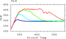
Figure 2: The relationship between surface temperature (K) and OLR (W/m²) for cases with various amounts of the non-condensable constituents are given. Blue: p_n0 = 10⁴ Pa. Aqua: p_n0 = 10⁵ Pa. Green: p_n0 = 10⁶ Pa. Red: p_n0 = 10⁷ Pa. The vertical grid resolution is that of L32.

Vertical Structures

It is confirmed that the value of OLR can be calculated accurately for p_n0 < 10⁶ Pa by L32. Here, we examine whether the vertical profiles of physical variables from L32 are also similar to those from L1000. Figures 3 and 4 show the vertical profiles of temperature and net upward radiative flux, respectively. The vertical profiles in both figures are similar to those from L1000, suggesting that L32 is also able to calculate the vertical structures with sufficient accuracy. In conclusion, we find that the use of L32 is sufficient for the purpose of calculating the atmospheric conditions with the present scheme for p_n0 = 10⁵ Pa and T_g ≤ 560 K.

(a) (b)

Figure 3: Vertical profiles of temperature (K) of 1D radiative solutions. (a) Results from L32. (b) Results from L1000. For p_n0=10⁵ Pa. The displayed results are for T_g = 250, 300, 350, 400, 450, 500, and 550 K.

(a) (b)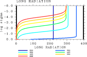

Figure 4: Vertical profiles of net upward radiative flux (W/m²) based on 1D radiative solutions. (a) Results from L32. (b) Results from L1000. For C_{Δ τ} = 0.1 and p_n0 = 10⁵ Pa. The displayed results are for T_g = 250, 300, 350, 400, 450, 500, and 550 K.

Summary

For radiation calculations, the use of 32 vertical layers is sufficient if p_n0 < 10⁶ Pa. However, this result represents merely the minimum number of vertical layers that is required in radiation calculation to obtain 1D equilibrium solutions. Additional investigations will be necessary to determine if the above result is applicable for atmospheric dynamics calculations. This topic will be addressed in future research.

C.c. Examination on the Vertical Resolution