4.4 Finite-Time Lyapunov Analysis on Fluid Deformation
Finite-time Lyapunov analysis ( Pierrehumbert,1991; Yoden and Nomura,1993 ) is done to evaluate quantitatively the stretching and mixing of fluid perticles.
Deformation field Ñu , or Jacobian matrix J can be
calculated in the same way as section 2.2 ,
in which the velocity field is given by (2.11)
of the line integration along the contour:
 (4.7)
(4.7)
During the evolution of the contour, time evolution of the tangent linear equation (2.17) is also calculated using (4.7) to obtain the resolvent M . Initial points are put on the grids of 200 x 200 .
The resolvent M is calculated for each initial point for several evaluation time τ, and finite-time Lyapunov exponents are obtained as the eigenvalues of MTM .


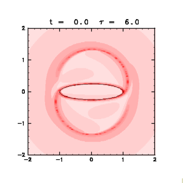
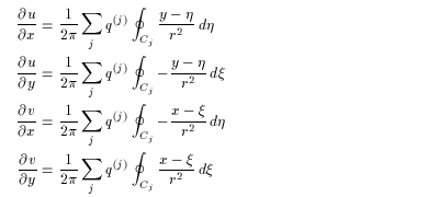
- The finite-time Lyapunov exponent is large not only on the contour but on the circle with its radius a little longer than the major axis of the elliptical vortex. The fluid particles in this region approach to a stagnation point to be streached out.
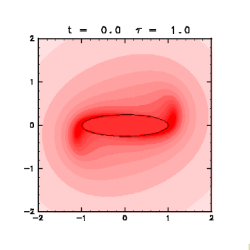
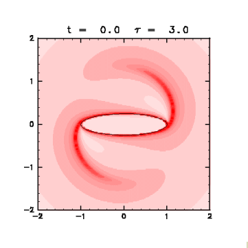
- As τ increases, two regions with large value on the circle are extended from the edge of the vortex. These regions reach the stagnation points within the evaluation time.
- On the other hand, the exponent is small inside the vortex, which is consistent with the facts that the fluid is separated from the outside, and that there exists little shear to stretch the fluid.
-
Moreover, the exponent is small also in two regions
slightly outside the minor axis of the ellipse.
These regions correspond to the regions of clockwise vortex
in the co-rotating frame with the vortex patch ( Fig. 5 ).
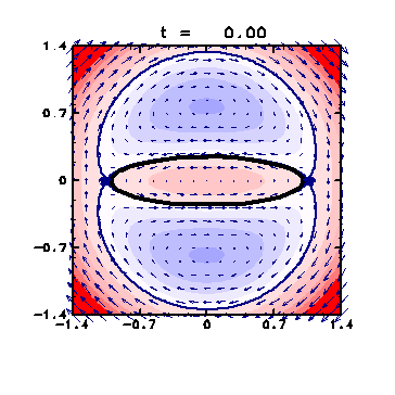 Figure 5: Velocity field in the co-rotating frame with the ellipse
(click for the expanded figure).
Figure 5: Velocity field in the co-rotating frame with the ellipse
(click for the expanded figure).
Same as Fig. 2 but the overall figure at t = 0 .