B. A Summary of One-Dimensional Radiative-Convective Equilibrium Modeling

b. Characteristics of One-Dimensional Radiative-Convective Equilibrium Solutions

Here, we will discuss on 1) the emitted radiation based on 1D radiative-convective equilibrium solutions and 2) the vertical structure of the equilibrium solutions.

One-Dimensional Radiative-Convective Equilibrium Model

We consider 1D radiative-convective equilibrium solutions for the case of a constant value of q in the stratosphere. In the troposphere, it is assumed that the temperature structure and water vapor content are determined from a moist adiabat. The 1D radiative-convective equilibrium solution is derived from the following procedure:

1. Assign a value to surface temperature, T_g.
2. Obtain surface pressure, p_s.
   The value of p_s is calculated from the following equation, using T_g.

   p_s = p_n0 + p^*_v (T_g).

   where p_n0 is the partial pressure of dry air (noncondensable constituents) at the bottom of the atmosphere and p^*_v (T_g) is the saturated water vapor pressure at the temperature T_g. With the use of the water vapor mixing ratio, q, ps can be expressed as
   $$p_s = P_n \times \{ 1 + q^* (T,p_n) \}$$

3. Obtain an adiabat structure from the surface.
   Assuming the adiabatic condition, the values of T_k and q_k = q^*(T_k) are determined starting at the surface (temperature: T_g; specific humidity: q^*(T_g) ) up to the highest layer. .
4. Calculate the radiative flux.
5. Evaluate the approximate value of the tropopause pressure.
   For the evaluation, it is assumed that the radiative flux is nearly constant within the upper layer of the troposphere and that this layer is in radiative equilibrium. It is also assumed that the tropopause is located roughly at the height at which the radiative flux starts to decrease.
6. Fine-tune the tropopause height.
   If the value of is positive, lower the tropopause height. In other words, if the air temperature evaluated with the assumption of radiative equilibrium is higher than the air temperature for the height under consideration, lower the tropopause height.
7. Once the position of the tropopause is determined, the layer above the tropopause (the stratosphere) is assumed to be in radiative equilibrium and q is set constant. The air temperature is then evaluated using

   $$\sigma T^4 = \frac{F^{\uparrow}_{top}}{2} \left(\frac{3}{2} \tau + 1 \right)$$

8. Recalculate the radiative flux.

The Relationship between Surface Temperature and OLR

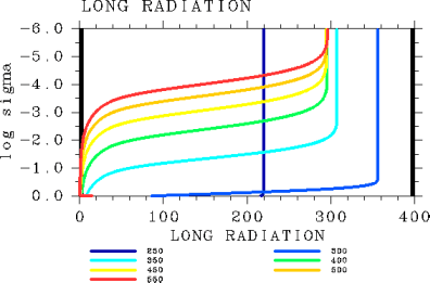
Figure 1 shows the relationship between surface temperature and OLR obtained from the 1D radiative-convective equilibrium model. This figure includes results from four cases in which the partial pressure of non-condensable atmospheric constituents, pn0, is set to 104, 105, 106, and 107 Pa. Figure 1 is characterized by the following features: A maximum value of OLR exists in all cases. With an increasing amount of non-condensable constituents, the maximum value of OLR increases and the curved OLR-ground temperature line becomes flat.

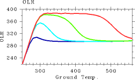
Figure 1: The relationship between surface temperature (K) and OLR (W/m2) of 1D radiative-convective equilibrium solutions. Blue: pn0 = 104 Pa. Aqua: pn0 = 105 Pa. Green: pn0 = 106 Pa. Red: pn0 = 107 Pa.

First, the surface temperature-OLR relationship is examined for the case of p_n0=10⁵ Pa. Refer to Nakajima et al. (1992) for details.

1. Cases of T_g ≤ 300 K
   In these cases, because total optical depth of the atmosphere does not exceed one, surface radiation σT_g⁴ contributes significantly to upward radiative flux. Thus, the value of OLR increases with increasing values of T_g. However, since the ground surface becomes invisible with increasing T_g, the rate of OLR increase becomes less pronounced .

2. Cases of 300 ≤ T_g ≤ 350 K
   In these cases, the relationship holds. Upward flux at the tropopause is primarily determined by the temperature structure of the middle layer of the troposphere. Because upward flux can be expressed as
   

   

   it can be presumed that OLR is determined by following term around

   $$\DD{}{\tau'} \pi B = 4 \sigma T^3 \DD{T}{\tau'}$$

   Accordingly, OLR tends to increase with an increasing temperature gradient around . Because q increases with increasing T_g, the temperature gradient approaches to an asymptotic value close to the moist-adiabatic lapse rate. Therefore, OLR decreases with increasing T_g. For the case in which OLR takes a value between 300 W/m² and 350 W/m², two equilibrium solutions exist. This circumstance arises since the same value of can be emitted by either a high-temperature stratosphere or the combination of a low-temperature troposphere and a low-temperature surface. The upper limit of in the cases of 300 ≤ T_g &lr; 350 K is 350 W/m², which is determined by the conditions of flux emissions from the troposphere.
3. Cases of T_g ≥ 350 K
   Because water vapor content in the troposphere increases significantly in these cases, the temperature structure of the troposphere can be determined from p^*(T). Therefore, both the value and gradient of T around become independent of T_g, thus only a single value is obtained for OLR regardless of the value of T_g. In these cases, is determined by the temperature structure of the middle layer of the troposphere. When the water vapor content becomes large (the temperature structure can be determined from the saturated water vapor pressure curve), and are approximately 305 W/m² and 300 W/m², respectively.

From the above discussions, the following conclusions can be reached. The value of OLR, i.e., , is determined according to upward radiation at the tropopause. However, an upper limit exists on radiation emitted from the troposphere, since it is determined from the water vapor profile as well as the temperature structure, which are set by the adiabatic condition. Accordingly, an upper limit also exists on the value of OLR. In the present paper, these limiting conditions will be referred to as the tropospheric flux emission conditions.

Subsequently, we will examine the trend that an increasing value of p_n0 leads to an increasing value of the maximum OLR and a plateauing of the value of OLR over a range of surface temperatures. When p_n0 increases, the relative amount of dry air increases, which causes the temperature gradient to approach the dry adiabatic lapse rate. As a result, the value of OLR becomes large. In fact, the numerical calculation results for a high value of p_n0 reveals little difference between the temperature structure of the troposphere and the dry adiabatic temperature structure.

The OLR-surface temperature line becomes flat for the following reason. From the relationship

$$d \tau = k q \frac{dp}{g}$$

the optical depth can be expressed as

$$\tau = \int^p_0 k q \frac{dp}{g}.$$

If it is assumed that the temperature structure of the troposphere is determined by the dry adiabatic lapse rate, then

$$\DD{T}{p} = \frac{1}{\rho C_p}$$

From this relationship, the vertical coordinate variable can be converted from T to p by neglecting the presence of the stratosphere and the relationship

$$\tau = \int^p_0 k q \frac{1}{g} \rho c_p dT.$$

can be obtained. Furthermore, the profile of water vapor which exists in a minute quantity is expressed as q = p^*(T)/p, and thus

$$\tau = \int^T_{T_{trop}} k p^{\ast} \frac{c_p}{g} dT.$$

Rearranging this equation, τ at an arbitrary T becomes

$$\tau(T) = \frac{k p_0 c_p}{g R} \int^T_0 \exp \left( - \frac{L}{RT} \right) \frac{dT}{T}$$

This equation shows that temperature can be uniquely determined once τ is given. Therefore, if the atmosphere is optically thick and the contribution by T_g can be neglected, only a single value of OLR is obtained regardless of the value of T_g.

Atmospheric Structure

Below, we will examine how the atmospheric structure of the 1D radiative-convective equilibrium solutions change according to the value of surface temperature. Here, the results from the case of p_n0 = 10⁵ Pa will be presented.

An examination of the vertical temperature profiles (Figure 2) shows that air temperature in the upper layer is the highest in the case of T_g = 300 K. The case with this air temperature coincides to the case with the maximum value of the OLR among the cases examined. Specific humidity approaches one across the entire layer with an increasing surface temperature (Figure 3). The layer undergoing radiative cooling is shifted to a higher altitude with an increasing surface temperature (Figure 6).

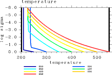
Figure 2: Vertical temperature profiles (K) for the case of p_n0 = 10⁵ Pa. The displayed results are for surface temperatures of 250, 300, 350, 400, 450, 500, and 550 K.

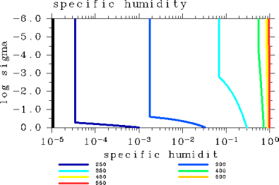
Figure 3: Vertical specific humidity profiles for the case of p_n0 = 10⁵ Pa. The displayed results are for surface temperatures of 250, 300, 350, 400, 450, 500, and 550 K.

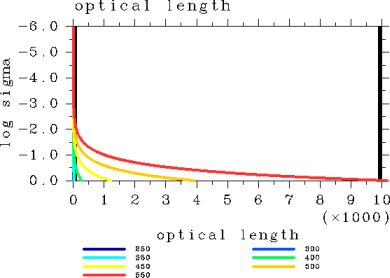
Figure 4: Vertical profiles of optical length for the case of p_n0 = 10⁵ Pa. The displayed results are for surface temperatures of 250, 300, 350, 400, 450, 500, and 550 K.<

Figure 5: Vertical profiles of net upward radiative flux (W/m²) for the case of p_n0 = 10⁵ Pa. The displayed results are for surface temperatures of 250, 300, 350, 400, 450, 500, and 550 K.

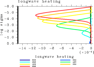
Figure 6: Vertical profiles of radiative heating rate (K/sec) for the case of p_n0 = 10⁵ Pa. The displayed results are for surface temperatures of 250, 300, 350, 400, 450, 500, and 550 K.

As inferred from above, the tropopause height increases with increasing surface temperature. Figure 7 illustrates the relationship between surface temperature and the tropopause height. As surface temperature increases, so does the water vapor content. This, in turn, increases the atmospheric mass. The relationship between surface temperature and surface pressure is depicted in Figure 8.

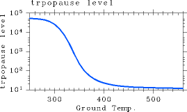
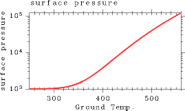
Figure 7: The dependency of tropopause pressure (Pa) on surface temperature (K). For the case of pn0 = 105 Pa. Figure 8: The dependency of surface pressure (Pa) on surface temperature (K). For the case of pn0 = 105 Pa.

B.b. Characteristics of One-Dimensional Radiative-Convective Equilibrium Solutions