A 2-dimensional non-divergent flow on a rotating sphere governed by the following vorticity equation will be examined.

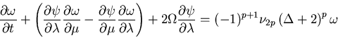
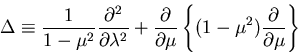
Here, ψ (λ, μ, t): stream functions; ω (λ, μ, t): vertical component of vorticity (≡ Δ ψ); λ: longitude; μ: sine latitude; t: time; Ω: angular speed of rotation of sphere; ν_2p: hyper-viscosity coefficient, and p: order of hyper-viscosity. Furthermore, Δ is the horizontal Laplacian and is defined as follows.

Note that,

• the dimensionless units of length and time are the radius of the sphere and a given time scale T, respectively,
• the above vorticity equation corresponds to the Lagrangian conservation law for potential vorticity of q ≡ ω + 2Ω μ in cases of inviscid fluids,
• the hyper-viscosity coefficient term on the right-hand side of the vorticity equation has been adopted for convenience to prevent numerical instability and failure, and
• the "+2" in the hyper-viscosity coefficient term on the right-hand side of the vorticity equation (Δ+2) has been added to conserve total angular momentum.

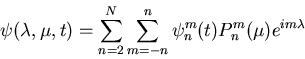
The dependent variable ψ is expanded using spherical harmonics as

where,

• P_n^m(μ) is the associated Legendre functions normalized by 2, and
• the reason the discretization starts from n = 2 is that the component of n = 1 corresponds to the total angular momentum, which is the conserved quantity in the vorticity equation.

Based on the above expansion, the simultaneous ordinary differential equations for the expansion coefficient ψ_n^m(t) is yielded from the vorticity equation using the spectral Galerkin method. The non-linear terms are calculated in real space, and a technique is adopted for returning the results back into the wavenumber space by Fourier-Legendre transformation. To eliminate aliasing, global surface domain is covered by a transform grid of 2,048 (longitudinal) × 1,024 (latitudinal) when the truncation wavenumber N = 682, and a grid of 1,024×512 when N = 341.

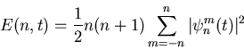
In the experiment for decaying turbulence, an initial turbulent field will be given to observe time evolution. The energy density is given by

The initial energy spectrum is constrained to be the distribution function employed by Cho and Polvani (1996)

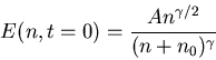
and each band wavenumber component m will be given random amplitude and phase. Here, coefficient A will be set so that the total dimensionless kinetic energy E_total ≡ Σ_n=2^NE(n,t=0) will be equal to 1. n₀ is a parameter that gives the central wavenumber, and will take the values of either 10, 50, or 100. γ is a parameter that determines the spectral width, and a larger value for γ will confine the initial energy to a narrower band. In the present study, γ was set to 1,000.

• The fact that E_total = 1 is adopted conversely implies that (radius of sphere) / √E_total has been adopted as the time scale for making the vorticity equation dimensionless.

The angular velocity of rotation Ω will be used as the experimental parameter and given six values, 0, 25, 50, 100, 200, and 400. When Ω ≠ 0, the planet will make Ω/(2π) rotations during unit time.

• In this scaling scheme, the relationship between dimensionless Ω and dimensional spherical radius of a^*, angular velocity of rotation of Ω^*, and mean wind velocity of U^* can be represented as Ω = √ 2 × a^*Ω^*/U^*. Since the model used in the present study is a 2-dimensional incompressible fluid, it is far from being a precise representation of the actual planetary atmosphere, but if forced to make analogies with actual conditions, the above values for Earth are a^* = 6.37×10⁶ m, Ω^* = 7.29×10^-5 s^-1, and if 15 ms^-1 is chosen for the value of U^*, then Ω = 43.8. For Jupiter, these values are a^* = 6.99×10⁷ m, Ω^* = 1.76×10^-4 s^-1, and if 50 ms^-1 is chosen for the value of U^*, then Ω = 348. Therefore, if we were to choose the results corresponding to the cases for Earth and Jupiter, then the experiments for Ω = 50 and Ω = 400 will roughly have parameters corresponding to that of Earth and Jupiter, respectively.

Note here that the wavenumber at which the non-linear term of the vorticity equation and the linear rotational effect term are nearly equal (wavenumber corresponding to the Rhines scale), n_β ≡ √ (π Ω/(4U))= √ (π Ω/(4√(2× E_total)) ) =√(π Ω/(4√ 2)), will be an important indicator. Actually, the manner of time evolution of the decaying turbulence is strongly dependent on the magnitude relation between n_β and the initial energy peak wavenumber n₀. When n_β > n₀, then the linear term will dominate over the non-linear term from the initial stages, and so the inverse energy cascade predicted by the turbulence theory will not always appear.

For the numerical viscosity term, p is set to 8, and ν_2p = 1×10^-43 (for N = 682), and 1×10^-38 (for N = 341). Time integration is done using the 4th-order Runge-Kutta method, with the time increment being set to Δt = 5×10^-4 (for N = 682) and 1×10^-3 (for N = 341), and time evolution will be computed to t = 5.

For the numerical calculations, the efficient transform code of ISPACK (ishioka, 1999) has been employed.

<<index <previous next>