Figure 3-2 (left panel) shows the typical horizontal structure of continuous modes for log E=-0.20, 4.35 ≤ c ≤ 4.67. A blue filled circle in right panel indicates the position of the mode. In this case, a north boundary Kelvin wave (N.B.K.) like structure and the structure of a continuous mode (C) are clearly observed. An equatorial Kelvin wave (K) like structure also seems to appear, although their amplitude are small.
The critical latitude for the mode shown in figure 3-2 is y=2.43. An amplitude peak of geopotential at y=2.40 shown in the left panel of figure 3-2 corresponds to the structure of continuous mode.
An amplitude peak of geopotential at y=3.00 is considered to correspond to a structure of north boundary Kelvin mode. The reasons are that phase speed of north boundary Kelvin mode is about 4 (indicated by an open triangle in the right panel of figure 3-2) which almost equals phase speed of the mode shown in figure 3-2, and that the structure trapped near the north boundary shows a boundary Kelvin wave like structure.
There is a possibility that structures of eastward inertial gravity modes and/or eastward mixed Rossby-gravity modes are mixing into the range of 2.00 < y < 3.00, since these eastward modes resonate with continuous modes at higher zonal wavenumber. However, only with figure 3-2, it is not confirmed that eastward inertial gravity modes and/or eastward mixed Rossby-gravity modes emerge in the horizontal structure of the continuous mode.
Velocity field near y=0 shows an equatorial Kelvin wave (K) like structure, although the amplitude is small. If equatorial Kelvin modes did not resonate with continuous modes, phase speed of neutral equatorial Kelvin modes would be about c=3.7 at k=0.10, which is smaller than phase speed of the continuous mode shown in figure 3-2. However, resonance with equatorial Kelvin modes and continuous modes seems to cause the mixing of equatorial Kelvin wave like structure into structures of continuous modes for wide range (ranging from figure 3-2 to figure 3-7).
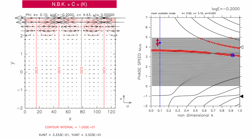
Figure 3-2: Horizontal strucutre of a continuous mode for log E=-0.20, k=0.10, c=4.43 (left panel). The position of the mode in dipspersion curves is indicated by a blue filled circle in the right panel. Contours and vectors in the left panel indicate &phi and velocity field, respectively. Contour intervals are 1.00 × 10⁻¹. Other symbols in the right panel are same as table 1.