Figure 3-4 (left panel) shows horizontal structure of unstable mode for log E=-0.20, c=3.65. A blue filled circle in right panel indicates the position of the mode. In this case, a north boundary Kelvin wave (N.B.K.) like structure and the structure of an unstable mode caused by resonance between equatorial Kelvin modes and continuous modes are observed.
The critical latitude of the mode shown in figure 3-4 is y=1.65. A deformation of the structure near y=1.70 is considered to be resulted from a continuous mode which resonates with equatorial Kelvin mode (similar deformation of structure can be observed in decaying mode with same phase speed, but figures are not shown here).
The amplitude peak of geopotential at y=0.00 shown in the left panel of figure 3-4 corresponds to equatorial Kelvin wave like structure. Kelvin wave mode resonates with continuous mode to cause the unstable mode shown in the figure (cf. TI2006).
The amplitude peak of geopotential at y=3.00 is considered to correspond to the structure of north boundary Kelvin mode. The reasons are that phase speed of north boundary Kelvin mode is about 4 (indicated by an open triangle in the right panel of figure 3-4) that almost equals phase speed of mode shown in left panel in figure 3-4, and that the structure trapped near the north boundary shows a boundary Kelvin wave like structure.
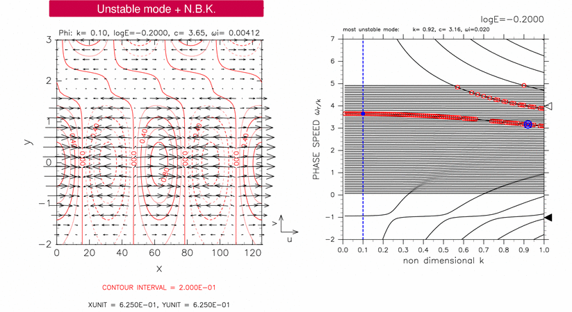
Figure 3-4: Horizontal structure of an unstable mode for log E=-0.20, k=0.10, c=3.65 (left panel). The position of the mode in dispersion curves is indicated by a blue filled circle in the right panel. Contours and vectors in the left panel indicate &phi and velocity field, respectively. Contour intervals are 2.00 × 10⁻¹. Other symbols in the right panel are same as table 1.