Figure 3-5 (left panel) shows the typical horizontal structure of continuous modes for log E=-0.20, 3.36 ≤ c ≤ 3.58. A blue filled circle in right panel indicates the position of the mode. In this case, a north boundary Kelvin wave (N.B.K.) like structure, the structure of a continuous mode (C), and an equatorial Kelvin wave (K) like structure are observed.
The critical latitude of the mode shown in figure 3-5 is y=1.50. The amplitude peak of geopotential at y=1.60 shown in the left panel of figure 3-5 corresponds to the structure of continuous mode.
A north boundary Kelvin wave like structure is observed at y=3.00. Although phase speed of north boundary Kelvin mode (indicated by an open triangle in the right panel of figure 3-5) is not close to phase speed of the mode shown in figure 3-5, north boundary Kelvin wave like structure is mixing into the continuous mode shown in this figure.
An equatorial Kelvin wave like structure appears around y=0.00. It is considered that an equatorial Kelvin wave like structure is mixing into the continuous mode for wide range of phase speed due to resonance with equatorial Kelvin modes and continuos modes.
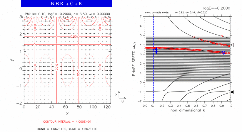
Figure 3-5: Horizontal structure of a continuous mode for log E=-0.20, k=0.10, c=3.50 (left panel). The position of the mode in dispersion curves is indicated by a blue filled circle in the right panel. Contours and vectors in the left panel indicate &phi and velocity field, respectively. Contour intervals are 4.00 × 10⁻¹. Other symbols in the right panel are same as table 1.