Figure 3-6 (left panel) shows the typical horizontal structure of continuous modes for log E=-0.20, 2.51 ≤ c ≤ 3.29. A blue filled circle in right panel indicates the position of the mode. In this case, a north boundary Kelvin wave (N.B.K.) like structure, an equatorial Rossby wave like structure (Rossby), and an equatorial Kelvin wave like structure (K) are observed. The structure of a continuous mode (C) cannot be identified.
The critical latitude of the mode shown in figure 3-6 is y=0.83. There should exist an amplitude peak of geopotential at y=0.83 corresponding to the structure of continuous mode, but such a peak cannot be observed in the left panel of figure 3-6. The structure of continuous mode is considered to be masked by an equatorial Rossby wave like structure described below.
A north boundary Kelvin wave like structure is observed at y=3.00. Although phase speed of north boundary Kelvin mode (indicated by an open triangle in the right panel of figure 3-6) is not close to phase speed of the mode shown in figure 3-6, north boundary Kelvin wave like structure is mixing into the continuous mode shown in this figure.
In 1.0 < y < 2.4, the structure shows geostrophic flow and seems to correspond to equatorial Rossby wave. Intrinsic phase speed (mode phase speed minus basic flow speed) in the region of 1.0 < y < 2.4 is negative, which is consistent with the characteristic of equatorial Rossby modes. However, in the region on the south of the dynamic equator, intrinsic phase speed is positive. It is considered that structures of equatorial Rossby mode are mixing into surrounding continuous modes in wide range of phase speed due to assimilation of equatorial Rossby modes into continuous modes for c < 2.5 as explained in figure 3-7.
The amplitude peak of geopotential at y=0.00 has a characteristics of equatorial Kelvin mode. If equatorial Kelvin modes did not resonate with continuous modes, phase speed of neutral equatorial Kelvin modes would be about c=3.7 at k=0.10, which is larger than phase speed of the continuous mode shown in figure 3-6. However, equatorial Kelvin wave like structures are mixing into structures of continuous modes for wide range as discussed in figure 3-2.
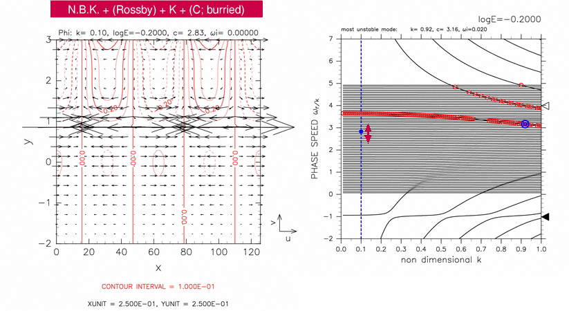
Figure 3-6: Horizontal structure of a continuous mode for log E=-0.20, k=0.10, c=2.83 (left panel). The position of the mode in dispersion curves is indicated by a blue filled circle in the right panel. Contours and vectors in the left panel indicate &phi and velocity field, respectively. Contour intervals are 1.00 × 10⁻¹. Other symbols in the right panel are same as table 1.