Figure 3-7 (left panel) shows the typical horizontal structure of continuous modes for log E=-0.20, 2.27 ≤ c ≤ 2.43. A blue filled circle in right panel indicates the position of the mode. In this case, a north boundary Kelvin wave (N.B.K.) like structure, an equatorial Rossby wave (Rossby) like structure, and an equatorial Kelvin wave (K) like structure are observed. The structure of a continuous mode (C) cannot be observed.
The critical latitude of the mode shown in figure 3-7 is y=0.35. There should exist an amplitude peak of geopotential at y=0.35 corresponding to the structure of continuous mode, but such a peak cannot be observed very well in the left panel of figure 3-7. The structure of continuous mode is considered to be masked by an equatorial Rossby wave like structure and an equatorial Kelvin wave like structure described below.
A north boundary Kelvin wave like structure is observed at y=3.00. Although phase speed of north boundary Kelvin mode (indicated by an open triangle in the right panel) is not close to phase speed of the mode shown in figure 3-7, north boundary Kelvin wave like structure is mixing into the continuous mode shown in this figure.
An amplitude peak of geopotential at y=1.60 is considered to be caused by equatorial Rossby mode. Since the dispersion curve of the mode shown in figure 3-7 exists between dispersion curves of equatorial Kelvin modes and westward mixed Rossby-gravity modes, equatorial Rossby modes is only candidate that produces the amplitude peak of geopotential at y=1.60. The geostrophic structure at y=1.60 shown in the left panel is also consistent with the existence of an equatorial Rossby mode.
The amplitude peak of geopotential at y=0.00 has a characteristics of equatorial Kelvin mode. Equatorial Kelvin wave like structures are mixing into structures of continuous modes for wide range as discussed in figure 3-2.
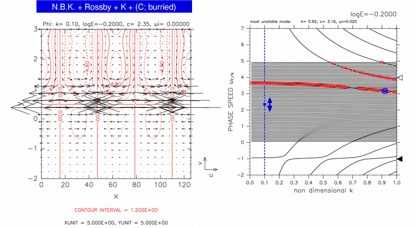
Figure 3-7: Horizontal structure of a continuous mode for log E=-0.20, k=0.10, c=2.35 (left panel). The position of the mode in dispersion curves is indicated by a blue filled circle in the right panel. Contours and vectors in the left panel indicate &phi and velocity field, respectively. Contour intervals are 1.20 × 100. Other symbols in the right panel are same as table 1.