5. Characteristic of neutral modes whose dispersion curves have intersection with other neutral modes

5.1 The objective of this section

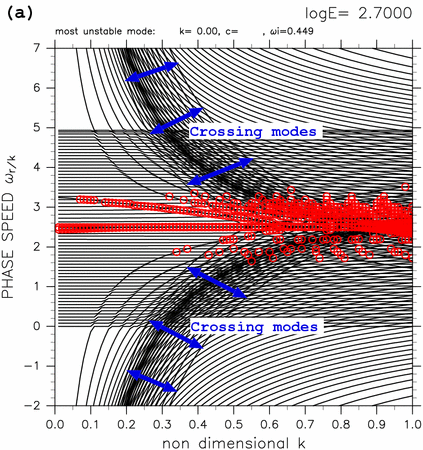
In dispersion relations obtained by TI2006 for large value of E, dispersion curves of some neutral modes intersect nearby dispersion curves of other neutral modes. An example of such intersection is shown in figure 6. Dispersion curves indicated by blue arrows, superimposed on dispersion curves of eastward (westward) inertial-gravity modes, intersect each other. In the followings, the modes whose dispersion curves intersect nearby curves are referred to as crossing modes. Crossing modes have following characteristics.

• Intersection with dispersion curves which have pseudomomentum with opposite sign does not cause instability. Continuous modes have negative pseudomomentum (Iga, 1999a), and eastward crossing modes indicated by blue arrows in figure 6 (a) and (b) have positive pseudomomentum (Iga, 1999b). Although instability is expected to occur by intersection of dispersion curves of these modes, any unstable mode does not appear (the result does not change in calculations with ten times higher resolution. Figures are not shown).
• Phase speed of crossing modes does not have asymptote of c=2.5 for large value of E. Phase speed of all equatorial waves in shear flow approach velocity of basic flow at dynamic equator in the limit of large E (Clark and Haynes, 1996). However, crossing modes have phase speed beyond the asymptotic value. Eastward crossing modes indicated by blue arrows in figure 6 have phase speed smaller than 2.5 for large wavenumber, and westward crossing modes have phase speed larger than 2.5 .

TI2006 did not mention those crossing modes. In this section, we examine crossing modes, and show their horizontal structures and existing condition.

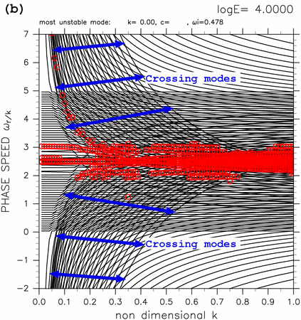Figure 6: Dispersion curves for (a) log E=+2.70, (b) log E=+4.00. Blue arrows indicate the region in which dispersion curves of crossing modes exist. Other symbols in the figures are same as table 1. Click above figures to show larger figures.

5.2 Existence condition for crossing modes

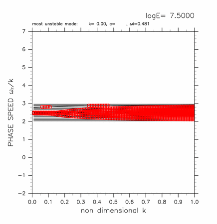
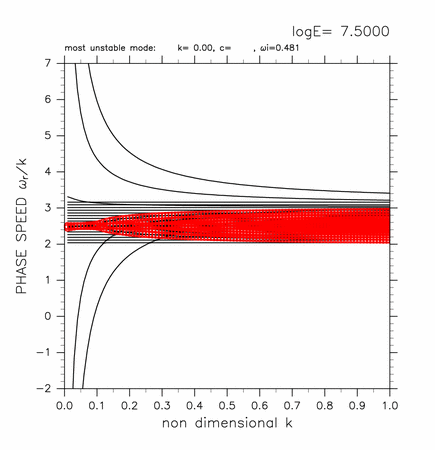
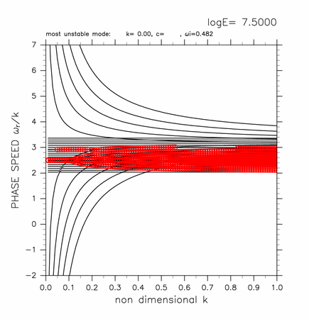
With calculations for various meridional width of computational domain, it is shown that the existence of computational domain outside the inertially unstable region causes crossing modes. Figure 7 shows a series of results in which computational domains are enlarged gradually from the case only with the inertially unstable region. The figure shows dispersion curves for large value of E, in which crossing modes, if they exist, can be observed clearly. The left panel of figure 7 shows the result for the case only with the inertially unstable region. In this case, no crossing mode emerges. The middle panel of figure 7 shows dispersion curves for the case in which two grid points exist on the north of the inertially unstable region. In this case, there exist two eastward crossing modes and two westward crossing modes. For the case of the right panel of figure 7, five grid points exist on the north of the inertially unstable region, and there exist five eastward crossing modes and five westward crossing modes. The results of other cases with various computational domain show that adding a grid point outside the inertially unstable region produces an eastward crossing mode, an westward crossing mode, and a continuous mode (Appendix B). On the other hand, crossing modes do not appear for the cases with only the inertially unstable region (0 ≤ y ≤ 1) regardless the number of grid points (Appendix C).

[Animation]	[Animation]	[Animation]

Figure 7: Dispersion curves for various meridional width of computational domain. (Left) 0.0 < y < 1.0, (Middle) 0.0 < y < 1.2, (Right) 0.0 < y < 1.4. The figures for log E=+7.50 are shown. Click each figure to show larger figure. Click [Animation] to show dispersion curves for various values of E. Refer to the caption of table 1 for the meanings of the symbols.

5.3 Horizontal structures of crossing modes

Figure 8 shows the result for log E=7.50 obtained with computational domain of 0.0 < y < 1.2. In this case, dispersion curves of crossing modes remain outside dispersion curves of continuous modes. The horizontal structure of the eastward crossing mode is shown in the left panel of figure 8. This figure shows that the crossing mode has large amplitude in the region of y > 1; outside the inertially unstable region. It is also confirmed that westward crossing mode has large amplitude in the region of y > 1 (see Appendix D). For smaller values of E, although dispersion curves of crossing modes do not intersect with other curves, crossing modes have large amplitude in the outside the inertially unstable region (see Appendix D). When computational domain exists on the north (south) of the inertially unstable region, both of eastward and westward crossing modes have large amplitude on the north (south) of the inertially unstable region. It is considered that crossing modes are gravity wave like modes existing in the channel region outside the inertially unstable region. Crossing modes are considered to be gravity wave like modes on a mid-latitude β-plane rather than equatorial wave modes.

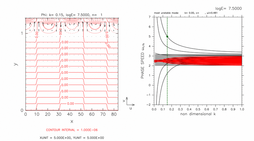
Figure 8: Horizontal structure (left) and dispersion curves (right) of crossing modes for log E=7.50, k=0.15 obtained with computational domain of 0 < y < 1.2. The position of the mode shown in left panel is indicated by green filled circles in right panel. Contours and vectors in the left panels indicate φ and the velocity field, respectively. Contour intervals (left) are 1.0 × 10^-6. Refer to the caption of table 1 for the meanings of symbols in right panels. Click figure to show larger figure.

5. Characteristic of neutral modes whose dispersion curves have intersection with other neutral modes